
 0000-0002-5865-6403
Stop using "Correlation is not causation" and maybe stop using correlation
- Introduction
- Linear correlation coefficient
- Zero correlation does not exclude causation
- Strictly linear relation only and robustness
- Geometric interpretation
- Non-linear interpretation and variance explained
- Non-random subsampling issue: correlation is subadditive
- Alternative measure for dependencies: Mutual Information
- On the independence of variables
- Conclusion: should I really stop using the correlation coefficient?
Introduction
We went from a world where the slightest correlation was treated as causation to a world where anytime the light is put on any correlation, it attracts a horde wielding “correlation is not causation” as a mantra, preventing any further thinking. The common point between the two aforementioned situations is that people still do not know the definition of correlation, independence and causation. By definition I do not mean only the mathematical definition, but also what these terms imply and their limits in practice.
In this article I will share some thoughts and examples to go further than the simple “correlation is not causation” slogan. I will also discuss if the concept of correlation is somehow useful, as observing directly a linear relationship is easier than interpreting the indicator itself. We will talk only about the problems related to the correlation coefficient: we will not discuss any model of causation1.
Future articles will cover more in depth the notions of independence, correlation, causality and the limits of \(p\)-value based science without proper causation model.
Linear correlation coefficient
Let us start with the definition of the correlation coefficient, or Pearson correlation coefficient, often simply referred as correlation.
Pearson correlation coefficient:
Given a pair of random variable \((X, Y)\), the correlation coefficient \(r\) is given by
with \(\text{cov}\) the covariance and \(\sigma\) the standard deviation.
The correletion takes value in \([-1, 1]\). As a first interpretation, one can notice that it is nothing but a normalized version of the covariance.
In practice, the correlation is often calculated on a sample of data. As \(\sigma_X^2 = \mathbb{E}[(X - \mathbb{E}[X])^2]\) and \(\text{cov}(X, Y) = \mathbb{E}[(X - \mathbb{E}[X])(Y - \mathbb{E}[Y])]\), we can rewrite the correlation as
And therefore, the sample correlation is calculated as
where \(\bar x\) and \(\bar y\) are the sample mean for \(X\) and \(Y\).
We will not talk about Spearman’s rank correlation despite most remarks applies.
Zero correlation does not exclude causation
Does the absence of correlation exclude causation?
Let’s start by something obvious but somehow often forgotten or unknown by the followers of the sect of correlation. The answer is no and let’s give few theoretical and practical counter-examples.
Example 1:
Assume a random variable \(Z\) following Rademacher law, that is to say taking values -1 and 1 with probability \(\frac 1 2\). Then define \(Y = ZX\) where \(X\) is any non-null random variable, independent from \(Z\). Then, correlation between \(X\) and \(Y\) is equal to \(0\) while obviously \(Y\) is not independent from \(X\) and fully caused by \(X\) and \(Z\).
Example 2:
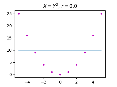
Another simple example: assume \(X\) following a uniform law on \([-1;1]\) and \(Y\) such that \(Y = X^2\). While \(Y\) is fully determined by \(X\), their correlation is 0.
Example 3: Cross-covariance
It holds also for cross-covariance:
Consider a sequence of \(N\) data points \(X = \{\begin{pmatrix} x_i \\ y_i \end{pmatrix}\}^N_{i=1}\) belonging to \(\mathbb{R}^2\) and consider a transformation \(g: \mathbb{R}^2 \mapsto \mathbb{R}^2\) defined by:
That is to say, \(g\) is a rotation by 90°. Now define \(Y = g(X)\). They cross-covariance is zero while again, both one sequence fully determines the second one.
Strictly linear relation only and robustness
Can correlation be used to automatically assess a linear relationship between variables? Can correlation measures non-linear relationships?
First of all, let us remind the reader that correlation usually refers to linear correlation, and therefore can only measure linear relations between variables. This is a hypothesis on the construction of the correlation coefficient itself. In other words, despite the fact that correlation can be calculated in any case, its validity in terms of interpretation is bounded by the fact that there is a linear relation between the variables.
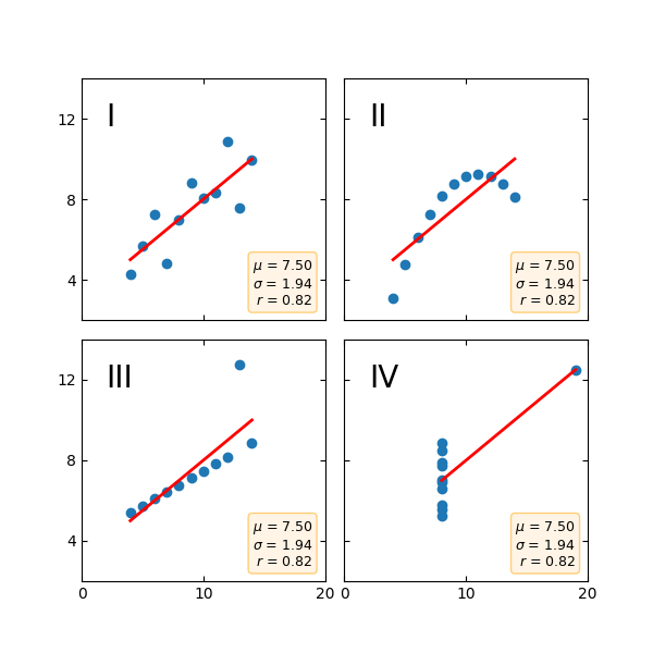
As a direct result, it is not enough to estimate the linear relationship by looking at the correlation coefficient: data must be visualized. This nullify the interest of using such coefficient to programmatically infer a linear relationship, and thus should be avoided in an AutoML setting. Indeed, it is easy to obtain a high correlation coefficient even with a non-linear relationship as illustrated by the following figure. The figure shows four datasets constructed by Francis Anscombe in 1973 to precisely demonstrate the importance of data visualization before analyzing it. This example goes beyond correlation because the mean and standard deviation are also all equal.
(Code originally from Matplotlib’s documentation)
Note again that the lack of linear relationship does not mean that there is no any other sort of non-linear relationship between the variable, and thus, potentially a causation relation, as demonstrated by quadrant II.
Observe also quadrant III: the correlation coefficient is a non-robust indicator of a linear relationship because an outlier can easily drastically and artificially lower its value. As a result, it is possible to downplay the importance of a linear relationship because of a single outlier. More generally, every model built on squared loss will be at risk of adversarial attack because adding a single well-engineered outlier might bias the model toward a desired outcome. Even without information about the gradient!
Of course, the impact of outliers is drastically reduced with large samples, or so-called big data. However, the complexity to visualize relationships increases with the dataset size and its dimensionality. So again, the conclusion here is that the correlation coefficient must be used carefully and discernment.
Geometric interpretation
How can I geometrically interpret the correlation?
Two sequences of points \(X = (x_{1},\ldots ,x_{n})\) and \(Y(y_{1},\ldots ,y_{n})\) can be considered as a vector in a \(n\) dimensional space. Denote by \({\bar {x}}\) the empiric average and consider the two centered vectors \(\bar X = (x_{1}-{\bar {x}},\ldots ,x_{n}-{\bar {x}})\) et \(\bar Y = (y_1 - \bar y, \ldots, y_n - \bar y)\).
The cosine value of the angle \(\alpha\) between the two centered vectors is given by:
Therefore, \(\cos(\alpha)= r_{p}\), which is why \(r\) always belongs to \([-1,1]\).
The correlation is nothing but the cosine of the angle between the two centered vectors:
- if \(r=1\), \(\alpha = 0\)
- if \(r=0\), \(\alpha = 90\)
- if \(r=-1\), \(\alpha = 180\)
Finally, the correlation coefficient can be interpreted not as a level of dependence between two variables but as their angular distance on the n-dimensional hypersphere. Way cooler to use, although probably inadequate to convince shareholders in a meeting about your future business plan.
Non-linear interpretation and variance explained
Assuming linear relationship between variables, is 0.5 to 0.6 the same as 0.8 to 0.9?
The answer is no. A correlation of 0.9 is vastly superior to 0.8. Same from 0.6 w.r.t. 0.5. However, the gap is much larger between 0.9 and 0.8 than it is between 0.6 and 0.5.
But the gap in what? If we take the square of the correlation coefficient, we obtain the coefficient of determination which can be interpreted as the variance of a variable \(X\) explained by another variable \(Y\).
In other words, another way of seeing the correlation coefficient is how well a linear regression explains the relation between two variables. Precisely, it evolves quadratically with the variance explained which is why its interpretation is not linear: variations close to 1 or -1 are more important than variations close to 0 and why 0.9 and vastly superior to 0.8.
Quantitatively speaking, the variance explained between 0.8 and 0.9 is, respectively, 64% and 81%, i.e. a 17 percentage points difference. On the contrary, between 0.5 and 0.6, the variance explained is, respectively, 25% and 36%, i.e. only 11pp.
Assuming a linear relationship, is 0.5 a good coefficient?
There are several considerations. If we study known-to-be-causal and stationary2 systems such as physical systems, then such correlation is insignificant because it is expected that the linear response to a linear system would lead to an almost perfect correlation coefficient (tainted by the uncertainty, measurement in particular).
Now, if we consider non-natural science, it might be tempting to say that due to the intrinsic complexity of, let’s say, social systems, with many variables, each with small individual impact, dynamics changing through time, most likely non-linear ones, with difficulties to isolate variables, etc. a lower correlation coefficient value of 0.5 or 0.6 is already something.
| \(r\) | \(r^2\) |
|---|---|
| 0. | 0. |
| 0.1 | 0.01 |
| 0.2 | 0.04 |
| 0.3 | 0.09 |
| 0.4 | 0.16 |
| 0.5 | 0.25 |
| 0.6 | 0.36 |
| 0.7 | 0.49 |
| 0.8 | 0.64 |
| 0.9 | 0.81 |
It surely is something, but not more than a possible starting point. As mentioned before, a correlation of 0.5 means that the variable explains 25% of the total observed variance. Usually, the purpose of a model is to explain a phenomena and/or to predict it.
With 25% variance explained, even assuming the existence of linear relationship, the predictive power of a simple linear model is very likely to be extremely poor.
Regarding the explanation power, it is not enough to decide. The linear relationship with the variable explains 25% of the observed variance:
- If the variable is the most impactful variable i.e. there is no variable that would explain more than 25%, then we have a mixed result: we have the most important variable (great!) but to explain more variance, as 25% is rather low, we would have to complexify our model. To reach a target of 75% variance explained, we would have to add at least three other variables, most likely more.
- If the variable is not the most impactful one, we are missing the big factor. Potentially from quite a lot since 75% of the variance remains to be explained. A scientist should NEVER be happy with a correlation coefficient close to 0.6 because of the possibility to fall in this category.
Non-random subsampling issue: correlation is subadditive
Correlation is subadditive. Consider two random variables \(X\) and \(Y\) whose joint distribution takes value in \(U = [0,1]^2\), and a partition of this space, arbitrarily \(U_1 = [0, 1] \times [0, \frac 1 2]\) and \(U_2 =[0, 1] \times [ \frac 1 2, 1]\). Then the following holds:
where \(w_i\) is the proportion of points from the total sample, i.e. \(\sum_i w_i = 1\).
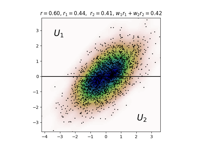
In other words, computing the correlation on subspaces and summing the results will always lead to underestimate the correlation. One might think it is enough to perform random sampling of \((X, Y)\) to get a proper estimation and avoid the weird idea to sample separate subspaces. The problem is that it works only for academic datasets and toy-models. In practice,
- We might not have enough information in advance to know the whole domain and data points mostly arrive sequentially.
- Data points coming sequentially might also not be sampled uniformely on \(U\) but on a restriction (independently of \(X\) and \(Y\)).
- And even when it is possible to request a sample, it might be very costly to do so in some regions of the domain, therefore introducing de facto a subspace.
- When I have access to external data, e.g. as a fact checker or journalist, I usually do not have information about whether the data are from a subsample or not.
Alternative measure for dependencies: Mutual Information
Can we measure nonlinear dependences?
Usually, people uses correlation as a measure of dependence, even if they know correlation is not causation.
Putting aside spurious correlations, their reasoning is as follows “if variables are not independent, then it means that they are somehow linked and influence each other - potentially by a confounding variable”. But as we have seen, the problem is that correlation measures only linear dependence.
There exist more general dependence measurements such as the Mutual Information, defined by
where \(D_{\mathrm {KL} }\) is the Kullback–Leibler divergence.
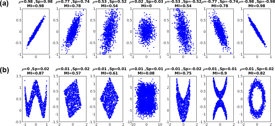
Computing it is not as easy as for the correlation, especially in practice where the joint distributions are not known and only a sample is available. Estimating the mutual information is currently actively being investigated. See for instance here, here or here. As illustrated in the following figure, the Mutual Information measures also nonlinear relationships.
It can actually be shown that the correlation coefficient can be directly connected to the Mutual Information in case \(X\) and \(Y\) is a bivariate normal distribution by:
with \(\begin{pmatrix} X \\ Y\end{pmatrix} \sim \mathcal{N}(\begin{pmatrix}\mu_1 \\ \mu_2\end{pmatrix}, \Sigma), ~ \Sigma = \begin{pmatrix} \sigma_1^2 & r\sigma_1\sigma_2\\ r\sigma_1\sigma_2& \sigma_2^2 \end{pmatrix}\)
More than the result itself, the actual information is that in general, one cannot infer the Mutual Information from the correlation or vice-versa.
On the independence of variables
The notion that a lot of people refer to when they think about correlation is actually the independence of two variables. We are getting further from the notion of causality, but roughly speaking, two events \(A\) and \(B\) are independent in the knowledge of one does not influence the second.
Mathematically, given \(A\) and \(B\) two events, \(A\) and \(B\) are independent iff \(\mathbb{P}(A \cap B) = \mathbb{P}(A) \mathbb{P}(B)\). It is probably more intuitive by considering that \(B\) is not null or not equals to one. Then \(A\) and \(B\) are independent implies that \(\mathbb{P}(A | B) = \mathbb{P}(A)\).
The problem is that we defined here, the independence of two events, not two random variables. Unfortunately, the proper definition of the independence of two or more random variables requires precise formalism which I would like to avoid here because it calls for an entire article by itself. Roughly speaking, a family of random variables defined on a probability space are independent if and only if the family of generated \(\sigma\)-algebra is itself independent.
In general, the independence of \(n\) events is difficult to apprehend. For instance, the pairwise independence of variables does not imply the independence of the family.
The two relations to keep in mind when talking about independence is:
- The absence of independence implies a zero correlation but zero correlation does not imply independence.
- Two variables being independent does not imply that there is an absence of causality between these variables.
Conclusion: should I really stop using the correlation coefficient?
No. For a single and very good reason: it is a measure of the amplitude of an effect. A linear effect precisely. It has many drawbacks, most of them being non-obvious. However, one of the main problems with the current standard scientific method is precisely that it is based on \(p\)-value which is NOT a measure of the amplitude of an effect but a purely binary threshold: either the effect is significant or not, with regards to an arbitrary threshold decided a priori. Contrarily to a common misconception, for a fixed threshold, let’s say \(0.05\), a \(p\)-value \(p_1 = 10^{-5}\) is not worse than a \(p\)-value \(p_2 = 10^{-10}\). It tells nothing about the amplitude of the effect. All it tells is that it would be far more surprising if the effect tested by \(p_2\) would not exist or be at random, compared to the effect tested by \(p_1\).
As a result, any indicator that can help to understand the amplitude of an effect is more than welcomed. The problem being, that in practice, many people are not taking into account the intrinsic limitations of such indicator.
In general, the correlation coefficient does not indicate whether:
- the independent variables are a cause of the changes in the dependent variable, that is to say, there are confounding factors,
- omitted-variable bias exists,
- the correct regression was used, that is to say, if the relation is indeed linear,
- the most appropriate set of independent variables has been chosen,
- there is collinearity present in the data on the explanatory variable,
- the model might be improved by using transformed versions of the existing set of independent variables,
- there are enough data points to make a solid conclusion.
In summary, linear correlation is the starting point of a reasoning, nothing more. An observation that should help us to look for an explanation or further results. It is not a golden measurement, it is rather hard to interprete compared to simply observing the phenomena it tries to measure. A lack of correlation does not mean there is no causation effect and a good correlation does not imply a causation effect. But at least, it is a measurement of the amplitude of an effect rather than a measure of how surprising it would be if an effect is due to randomness, and just for this, you should continue to use it with parsimony.
-
To be honest, I decided to write this article just before reading The Book of Why by Judea Pearl, as an exercise to compared my understanding of causation before and after. ↩
-
Systems such that their dynamic does not evolve in time. We could also include systems such that the dynamic might evolve by actions performed by the observers but not systems whose dynamic evolves according to an unobserved and unknown law. ↩